Table of Contents
It is always best to start simply. And since lighting is a big topic, we will begin with the simplest possible scenario.
Lighting is complicated. Very complicated. The interaction between a surface and a light is mostly well understood in terms of the physics. But actually doing the computations for full light/surface interaction as it is currently understood is prohibitively expensive.
As such, all lighting in any real-time application is some form of approximation of the real world. How accurate that approximation is generally determines how close to photorealism one gets. Photorealism is the ability to render a scene that is indistinguishable from a photograph of reality.
Non-Photorealistic Rendering
There are lighting models that do not attempt to model reality. These are, as a group, called non-photorealistic rendering (NPR) techniques. These lighting models and rendering techniques can attempt to model cartoon styles (typically called “cel shading”), paintbrush effects, pencil-sketch, or other similar things. NPR techniques including lighting models, but they also do other, non-lighting things, like drawing object silhouettes in an dark, ink-like color.
Developing good NPR techniques is at least as difficult as developing good photorealistic lighting models. For the most part, in this book, we will focus on approximating photorealism.
A lighting model is an algorithm, a mathematical function, that determines how a surface interacts with light.
In the real world, our eyes see by detecting light that hits them. The structure of our iris and lenses use a number of photorecepters (light-sensitive cells) to resolve a pair of images. The light we see can have one of two sources. A light emitting object like the sun or a lamp can emit light that is directly captured by our eyes. Or a surface can reflect light from another source that is captured by our eyes. Light emitting objects are called light sources.
The interaction between a light and a surface is the most important part of a lighting model. It is also the most difficult to get right. The way light interacts with atoms on a surface alone involves complicated quantum mechanical principles that are difficult to understand. And even that does not get into the fact that surfaces are not perfectly smooth or perfectly opaque.
This is made more complicated by the fact that light itself is not one thing. There is no such thing as “white light.” Virtually all light is made up of a number of different wavelengths. Each wavelength (in the visible spectrum) represents a color. White light is made of many wavelengths (colors) of light. Colored light simply has fewer wavelengths in it than pure white light.
Surfaces interact with light of different wavelengths in different ways. As a simplification of this complex interaction, we will assume that a surface can do one of two things: absorb that wavelength of light or reflect it.
A surface looks blue under white light because the surface absorbs all non-blue parts of the light and only reflects the blue parts. If one were to shine a red light on the surface, the surface would appear very dark, as the surface absorbs non-blue light, and the red light does not have much blue light in it.

Therefore, the apparent color of a surface is a combination of the absorbing characteristics of the surface (which wavelengths are absorbed or reflected) and the wavelengths of light shone upon that surface.
The very first approximation that is made is that not all of these wavelengths matter. Instead of tracking millions of wavelengths in the visible spectrum, we will instead track 3. Red, green, and blue.
The RGB intensity of light reflected from a surface at a particular point is a combination of the RGB light absorbing characteristics of the surface at that point and the RGB light intensity shone on that point on the surface. All of these, the reflected light, the source light, and the surface absorption, can be described as RGB colors, on the range [0, 1].
The intensity of light shone upon a surface depends on (at least) two things. First, it depends on the intensity of light that reaches the surface from a light source. And second, it depends on the angle between the surface and the light.
Consider a perfectly flat surface. If you shine a column of light with a known intensity directly onto that surface, the intensity of that light at each point under the surface will be a known value, based on the intensity of the light divided by the area projected on the surface.

If the light is shone instead at an angle, the area on the surface is much wider. This spreads the same light intensity over a larger area of the surface; as a result, each point under the light “sees” the light less intensely.

Therefore, the intensity of the light cast upon a surface is a function of the original light's intensity and the angle between the surface and the light source. This angle is called the angle of incidence of the light.
A lighting model is a function of all of these parameters. This is far from a comprehensive list of lighting parameters; this list will be expanded considerably in future discussions.
Diffuse lighting refers to a particular kind of light/surface interaction, where the light from the light source reflects from the surface at many angles, instead of as a perfect mirror.

An ideal diffuse material will reflect light evenly in all directions, as shown in the picture above. No actual surfaces are ideal diffuse materials, but this is a good starting point and looks pretty decent.
For this tutorial, we will be using the Lambertian reflectance model of diffuse lighting. It represents the ideal case shown above, where light is reflected in all directions equally. The equation for this lighting model is quite simple:

The cosine of the angle of incidence is used because it represents the perfect hemisphere of light that would be reflected. When the angle of incidence is 0°, the cosine of this angle will be 1.0. The lighting will be at its brightest. When the angle of incidence is 90°, the cosine of this angle will be 0.0, so the lighting will be 0. Values less than 0 are clamped to 0.
Now that we know what we need to compute, the question becomes how to compute it. Specifically, this means how to compute the angle of incidence for the light, but it also means where to perform the lighting computations.
Since our mesh geometry is made of triangles, each individual triangle is flat. Therefore, much like the plane above, each triangle faces a single direction. This direction is called the surface normal or normal. It is the direction that the surface is facing at the location of interest.
Every point along the surface of a single triangle has the same geometric surface normal. That's all well and good, for actual triangles. But polygonal models are usually supposed to be approximations of real, curved surfaces. If we use the actual triangle's surface normal for all of the points on a triangle, the object would look very faceted. This would certainly be an accurate representation of the actual triangular mesh, but it reveals the surface to be exactly what it is: a triangular mesh approximation of a curved surface. If we want to create the illusion that the surface really is curved, we need to do something else.
Instead of using the triangle's normal, we can assign to each vertex the normal that it would have had on the surface it is approximating. That is, while the mesh is an approximation, the normal for a vertex is the actual normal for that surface. This actually works out surprisingly well.
This means that we must add to the vertex's information. In past tutorials, we have had a position and sometimes a color. To that information, we add a normal. So we will need a vertex attribute that represents the normal.
So each vertex has a normal. That is useful, but it is not sufficient, for one simple reason. We do not draw the vertices of triangles; we draw the interior of a triangle through rasterization.
There are several ways to go about computing lighting across the surface of a triangle. The simplest to code, and most efficient for rendering, is to perform the lighting computations at every vertex, and then let the result of this computation be interpolated across the surface of the triangle. This process is called Gouraud shading.
Gouraud shading is a pretty decent approximation, when using the diffuse lighting model. It usually looks OK so long as we remain using that lighting model, and was commonly used for a good decade or so. Interpolation of vertex outputs is a very fast process, and not having to compute lighting at every fragment generated from the triangle raises the performance substantially.
That being said, modern games have essentially abandoned this technique. Part of that is because the per-fragment computation is not as slow and limited as it used to be. And part of it is simply that games tend to not use just diffuse lighting anymore, so the Gouraud approximation is more noticeably inaccurate.
The angle of incidence is the angle between the surface normal and the direction towards the light. Computing the direction from the point in question to the light can be done in a couple of ways.
If you have a light source that is very close to an object, then the direction towards the light can change dramatically over the surface of that object. As the light source is moved farther and farther away, the direction towards the light varies less and less over the surface of the object.

If the light source is sufficiently distant, relative to the size of the scene being rendered, then the direction towards the light is nearly the same for every point on every object you render. Since the direction is the same everywhere, the light can be represented as just a single direction given to all of the objects. There is no need to compute the direction based on the position of the point being illuminated.
This situation is called a directional light source. Light from such a source effectively comes from a particular direction as a wall of intensity, evenly distributed over the scene.
Direction light sources are a good model for lights like the sun relative to a small region of the Earth. It would not be a good model for the sun relative to the rest of the solar system. So scale is important.
Light sources do not have to be physical objects rendered in the scene. All we need to use a directional light is to provide a direction to our lighting model when rendering the surface we want to see. However, having light appear from seemingly nothing hurts verisimilitude; this should be avoided where possible.
Alternatives to directional lights will be discussed a bit later.
Normals have many properties that positions do. Normals are vector directions, so like position vectors, they exist in a certain coordinate system. It is usually a good idea to have the normals for your vertices be in the same coordinate system as the positions in those vertices. So that means model space.
This also means that normals must be transformed from model space to another space. That other space needs to be the same space that the lighting direction is in; otherwise, the two vectors cannot be compared. One might think that world space is a fine choice. After all, the light direction is already defined in world space.
You certainly could use world space to do lighting. However, for our purposes, we will use camera space. The reason for this is partially illustrative: in later tutorials, we are going to do lighting in some rather unusual spaces. By using camera space, it gets us in the habit of transforming both our light direction and the surface normals into different spaces.
We will talk more in later sections about exactly how we transform the normal. For now, we will just transform it with the regular transformation matrix.
The full lighting model for computing the diffuse reflectance from directional light sources, using per-vertex normals and Gouraud shading, is as follows. The light will be represented by a direction and a light intensity (color). The light direction passed to our shader is expected to be in camera space already, so the shader is not responsible for this transformation. For each vertex (in addition to the normal position transform), we:
Transform the normal from model space to camera space using the model-to-camera transformation matrix.
Compute the cosine of the angle of incidence.
Multiply the light intensity by the cosine of the angle of incidence, and multiply that by the diffuse surface color.
Pass this value as a vertex shader output, which will be written to the screen by the fragment shader.
This is what we do in the Basic Lighting tutorial. It renders a cylinder above a flat plane, with a single directional light source illuminating both objects. One of the nice things about a cylinder is that it has both curved and flat surfaces, thus making an adequate demonstration of how light interacts with a surface.
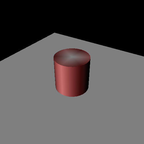
The light is at a fixed direction; the model and camera both can be rotated.
Pressing the Spacebar will switch between a cylinder that has a varying diffuse color and one that is pure white. This demonstrates the effect of lighting on a changing diffuse color.
The initialization code does the usual: loads the shaders, gets uniforms from them, and loads a number of meshes. In this case, it loads a mesh for the ground plane and a mesh for the cylinder. Both of these meshes have normals at each vertex; we'll look at the mesh data a bit later.
The display code has gone through a few changes. The vertex shader uses only two matrices: one for model-to-camera, and one for camera-to-clip-space. So our matrix stack will have the camera matrix at the very bottom.
Example 9.1. Display Camera Code
glutil::MatrixStack modelMatrix;
modelMatrix.SetMatrix(g_viewPole.CalcMatrix());

glm::vec4 lightDirCameraSpace = modelMatrix.Top() * g_lightDirection;

glUseProgram(g_WhiteDiffuseColor.theProgram);
glUniform3fv(g_WhiteDiffuseColor.dirToLightUnif, 1, glm::value_ptr(lightDirCameraSpace));
glUseProgram(g_VertexDiffuseColor.theProgram);
glUniform3fv(g_VertexDiffuseColor.dirToLightUnif, 1, glm::value_ptr(lightDirCameraSpace));
glUseProgram(0);
Since our vertex shader will be doing all of its lighting computations in camera
space, we need to move the g_lightDirection from world space to
camera space. So we multiply it by the camera matrix. Notice that the camera matrix
now comes from the MousePole object.
Now, we need to talk a bit about vector transforms with matrices. When transforming positions, the fourth component was 1.0; this was used so that the translation component of the matrix transformation would be added to each position.
Normals represent directions, not absolute positions. And while rotating or scaling a direction is a reasonable operation, translating it is not. Now, we could just adjust the matrix to remove all translations before transforming our light into camera space. But that's highly unnecessary; we can simply put 0.0 in the fourth component of the direction. This will do the same job, only we do not have to mess with the matrix to do so.
This also allows us to use the same transformation matrix for vectors as for positions.
We upload the camera-space light direction to the two programs.
To render the ground plane, we run this code:
Example 9.2. Ground Plane Lighting
glutil::PushStack push(modelMatrix);

glUseProgram(g_WhiteDiffuseColor.theProgram);
glUniformMatrix4fv(g_WhiteDiffuseColor.modelToCameraMatrixUnif, 1, GL_FALSE, glm::value_ptr(modelMatrix.Top()));
glm::mat3 normMatrix(modelMatrix.Top());
glUniformMatrix3fv(g_WhiteDiffuseColor.normalModelToCameraMatrixUnif, 1, GL_FALSE, glm::value_ptr(normMatrix));
glUniform4f(g_WhiteDiffuseColor.lightIntensityUnif, 1.0f, 1.0f, 1.0f, 1.0f);
g_pPlaneMesh->Render();
glUseProgram(0);
We upload two matrices. One of these is used for normals, and the other is used for positions. The normal matrix is only 3x3 instead of the usual 4x4. This is because normals do not use the translation component. We could have used the trick we used earlier, where we use a 0.0 as the W component of a 4 component normal. But instead, we just extract the top-left 3x3 area of the model-to-camera matrix and send that.
Of course, the matrix is the same as the model-to-camera, except for the lack of translation. The reason for having separate matrices will come into play later.
We also upload the intensity of the light, as a pure-white light at full brightness. Then we render the mesh.
To render the cylinder, we run this code:
Example 9.3. Cylinder Lighting
glutil::PushStack push(modelMatrix);

modelMatrix.ApplyMatrix(g_objtPole.CalcMatrix());

if(g_bDrawColoredCyl)
{
    glUseProgram(g_VertexDiffuseColor.theProgram);
    glUniformMatrix4fv(g_VertexDiffuseColor.modelToCameraMatrixUnif, 1, GL_FALSE, glm::value_ptr(modelMatrix.Top()));
    glm::mat3 normMatrix(modelMatrix.Top());
    glUniformMatrix3fv(g_VertexDiffuseColor.normalModelToCameraMatrixUnif, 1, GL_FALSE, glm::value_ptr(normMatrix));
    glUniform4f(g_VertexDiffuseColor.lightIntensityUnif, 1.0f, 1.0f, 1.0f, 1.0f);
    g_pCylinderMesh->Render("lit-color");
}
else
{
    glUseProgram(g_WhiteDiffuseColor.theProgram);
    glUniformMatrix4fv(g_WhiteDiffuseColor.modelToCameraMatrixUnif, 1, GL_FALSE, glm::value_ptr(modelMatrix.Top()));
    glm::mat3 normMatrix(modelMatrix.Top());
    glUniformMatrix3fv(g_WhiteDiffuseColor.normalModelToCameraMatrixUnif, 1, GL_FALSE, glm::value_ptr(normMatrix));
    glUniform4f(g_WhiteDiffuseColor.lightIntensityUnif, 1.0f, 1.0f, 1.0f, 1.0f);
    g_pCylinderMesh->Render("lit");
}
glUseProgram(0);
The cylinder is not scaled at all. It is one unit from top to bottom, and the diameter of the cylinder is also 1. Translating it up by 0.5 simply moves it to being on top of the ground plane. Then we apply a rotation to it, based on user inputs.
We actually draw two different kinds of cylinders, based on user input. The colored cylinder is tinted red and is the initial cylinder. The white cylinder uses a vertex program that does not use per-vertex colors for the diffuse color; instead, it uses a hard-coded color of full white. These both come from the same mesh file, but have special names to differentiate between them.
What changes is that the “flat” mesh does not pass the color vertex attribute and the “tint” mesh does.
Other than which program is used to render them and what mesh name they use, they are both rendered similarly.
The camera-to-clip matrix is uploaded to the programs in the
reshape function, as previous tutorials have
demonstrated.
There are two vertex shaders used in this tutorial. One of them uses a color
vertex attribute as the diffuse color, and the other assumes the diffuse color is
(1, 1, 1, 1). Here is the vertex shader that uses the color attribute,
DirVertexLighting_PCN:
Example 9.4. Lighting Vertex Shader
#version 330

layout(location = 0) in vec3 position;
layout(location = 1) in vec4 diffuseColor;
layout(location = 2) in vec3 normal;

smooth out vec4 interpColor;

uniform vec3 dirToLight;
uniform vec4 lightIntensity;

uniform mat4 modelToCameraMatrix;
uniform mat3 normalModelToCameraMatrix;

layout(std140) uniform Projection
{
    mat4 cameraToClipMatrix;
};

void main()
{
    gl_Position = cameraToClipMatrix * (modelToCameraMatrix * vec4(position, 1.0));

	vec3 normCamSpace = normalize(normalModelToCameraMatrix * normal);

    float cosAngIncidence = dot(normCamSpace, dirToLight);
    cosAngIncidence = clamp(cosAngIncidence, 0, 1);

    interpColor = lightIntensity * diffuseColor * cosAngIncidence;
}
We define a single output variable, interpColor, which will be
interpolated across the surface of the triangle. We have a uniform for the
camera-space lighting direction dirToLight. Notice the name: it
is the direction from the surface towards the light. It is not
the direction from the light.
We also have a light intensity uniform value, as well as two matrices for
positions and a separate one for normals. Notice that the
cameraToClipMatrix is in a uniform block. This allows us to
update all programs that use the projection matrix just by changing the buffer
object.
The first line of main simply does the position transforms we
need to position our vertices, as we have seen before. We do not need to store the
camera-space position, so we can do the entire transformation in a single
step.
The next line takes our normal and transforms it by the model-to-camera matrix
specifically for normals. As noted earlier, the contents of this matrix are
identical to the contents of modelToCameraMatrix. The
normalize function takes the result of the transform and
ensures that the normal has a length of one. The need for this will be explained
later.
We then compute the cosine of the angle of incidence. We'll explain how this math
computes this shortly. Do note that after computing the cosine of the angle of
incidence, we then clamp the value to between 0 and 1 using the GLSL built-in
function clamp.
This is important, because the cosine of the angle of incidence can be negative. This is for values which are pointed directly away from the light, such as the underside of the ground plane, or any part of the cylinder that is facing away from the light. The lighting computations do not make sense with this value being negative, so the clamping is necessary.
After computing that value, we multiply it by the light intensity and diffuse color. This result is then passed to the interpolated output color. The fragment shader is a simple passthrough shader that writes the interpolated color directly.
The version of the vertex shader without the per-vertex color attribute simply
omits the multiplication with the diffuseColor (as well as the
definition of that input variable). This is the same as doing a multiply with a
color vector of all 1.0.
We glossed over an important point in looking at the vertex shader. Namely, how the cosine of the angle of incidence is computed.
Given two vectors, one could certainly compute the angle of incidence, then take the cosine of it. But both computing that angle and taking its cosine are quite expensive. Instead, we elect to use a vector math trick: the vector dot product.
The vector dot product between two vectors can be mathematically computed as follows:

If both vectors have a length of one (ie: they are unit vectors), then the result of a dot product is just the cosine of the angle between the vectors.
This is also part of the reason why the light direction is the direction towards the light rather than from the light. Otherwise we would have to negate the vector before performing the dot product.
What makes this faster than taking the cosine of the angle directly is that, while the dot product is geometrically the cosine of the angle between the two unit vectors, computing the dot product via vector math is very simple:

This does not require any messy cosine transcendental math computations. This does not require using trigonometry to compute the angle between the two vectors. Simple multiplications and additions; most graphics hardware can do billions of these a second.
Obviously, the GLSL function dot computes the vector dot
product of its arguments.